Why your revenue forecast breaks when customers control the meter

In a subscription business, the forecast is simple in shape. It is new bookings from the pipeline, plus renewal and expansion of a contractually anchored base. The contract sets the number. The forecast tracks the contract.

In a consumption business, the existing-customer base is the dominant driver, and its behavior is variable by design. A single large customer's engineering decision can move a quarter. Adopting a new workload, pausing a project, or shifting to another provider all land straight in revenue. That one decision can outweigh the entire new-logo pipeline.

This is why contracted-revenue metrics are weak forward indicators here. Snowflake makes the point in its own filings. Its fiscal-2025 annual report covers the year ended January 31, 2025. In it, the company states that remaining performance obligations are not necessarily indicative of future product revenue. The reason it gives is that the figure ignores the timing of customer consumption. The same disclosure persists through its fiscal-2026 full-year results, reported in February 2026. Snowflake also describes forecasting future revenue with predictive models built on customers' historical usage. That is a consumption vendor telling investors, in its own filings, that usage models are how it plans.

Existing-base consumption typically dominates total revenue in a mature usage-based business. The exact share varies by company, so treat it as a structural fact, not a fixed percentage. The forecasting implication holds either way. Most of next quarter's revenue already sits inside your customer base, waiting to be modeled from how those customers behave.

Before building anything, answer four questions. They place your forecast and tell you which parts are firm.

1. What share of next quarter's revenue is contractually committed versus consumption-driven? That sets how much of the forecast is already firm.

2. How many quarters of usage actuals do you have? That places you on the maturity curve below.

3. Do you have redemption history for prepaid credits? That decides whether breakage can enter the forecast at all.

4. How concentrated is usage in your top accounts? That decides whether a point estimate is safe or a scenario range is required.

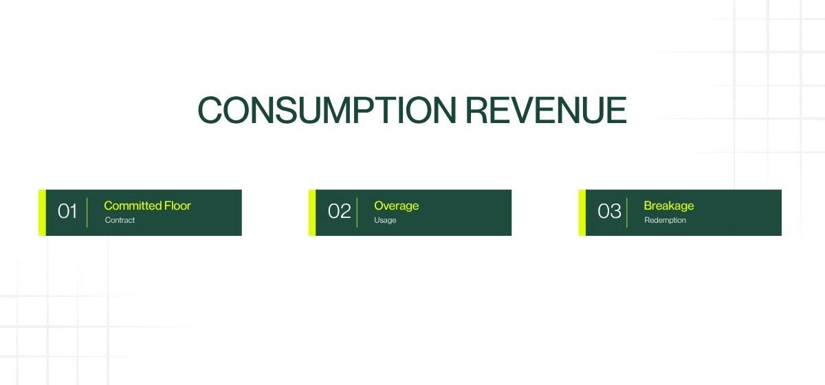
Stop forecasting consumption revenue as one number. Break it into three layers. Each has a different source of truth and a different level of predictability.

The committed floor. This is revenue from contractual minimums. It is predictable, contractually backed, and forecastable straight from the contract database. The caution: the floor is not always a fixed number. True-ups and ramp schedules can change it period to period. Pull every contract with a minimum, build the floor schedule, and confirm with deal desk or legal whether any true-up or ramp provisions move it.

The overage layer. This is revenue from consumption above the minimum. It is the demand-modeling component, built from account-level usage history, cohort ramp curves, and the leading indicators below.

Two cautions matter here. First, overage is not a fixed percentage of the floor. It is driven by adoption velocity, which varies by customer, workload, and season. Second, watch the pricing curve. When rates are tiered or decline with volume, more tokens do not mean proportionally more revenue. A model that multiplies projected volume by a headline rate will over-forecast revenue once customers cross into lower-priced tiers. Model the rate steps, not just the volume.

A recognition note matters for how the forecast maps to booked revenue. Much consumption usage is a single performance obligation satisfied over time. It is a series of substantially similar increments transferred in the same pattern, recognized as the customer consumes. This is why the overage forecast, a demand model, and recognized overage revenue, usage as it occurs, track each other closely. The committed floor and any bundled distinct promises may recognize on a different pattern. Know which elements recognize as a usage series and which do not, because they behave differently in the model.

The breakage layer. This is revenue from prepaid credits that expire unused. It is the layer most often modeled wrong, so it is worth stating the standard plainly.

Breakage is not a policy choice between a proportional method and a remote method. The treatment depends on whether the company expects to be entitled to the breakage. If it expects to be entitled, it estimates the amount. It then recognizes that amount in proportion to the pattern of rights the customer exercises, as credits are consumed. If it does not expect to be entitled, it recognizes breakage only when the likelihood of the customer using the remaining credits becomes remote.

Two guardrails belong in the forecast. First, the constraint. Breakage is variable consideration. The forecast can include it only up to the level where a significant revenue reversal is not probable once the uncertainty resolves. A company with thin redemption history may find its breakage estimate constrained, sometimes to zero, until it has enough data. Second, escheatment. Any portion of unused credits the company must remit to a government under unclaimed property law is a liability, not revenue. It never enters the breakage estimate.

So model the breakage layer from historical redemption patterns where they exist. Apply the constraint so the forecast does not book breakage the standard would not yet allow. Carve out escheatable amounts entirely.

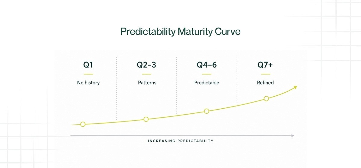
The honest answer to "can you forecast this?" depends on how much history you have. Predictability is not a switch. It is a curve. Here is where a company sits at each stage.

Quarter 1, no history. You have no usage data to model from. Forecast the committed floor with confidence. Express overage as a range, not a point estimate. Constrain breakage heavily, often to zero, given the absence of redemption history. Tell the board the range will narrow as data arrives. That is honest, not weak.

Quarters 2 to 3, first patterns. With a quarter or two of actuals, the first cohort ramp curves appear. You can see how fast new accounts reach steady-state usage, and at what level. Early seasonal signals may surface. Replace the sales-team overage guess with a cohort-based projection, grouped by start date and contract size. Still rough, but now data-driven.

Quarters 4 to 6, predictability establishes. With a year of data, cohort decay and stabilization rates become measurable. Seasonality is confirmed or rejected. Redemption history may finally support a breakage estimate that survives the constraint. Leading indicators become genuinely predictive. You can backtest the three-layer model against actuals, and the backtest exposes biases to correct. Accuracy reaches the point where the board can use it for guidance.

Quarter 7 and beyond, refinement. The model is stable. The work shifts to segmentation by workload, churn-risk prediction from usage-velocity decline, and narrowing the confidence interval. The forecast becomes a living tool, refreshed as usage data arrives, not a quarterly scramble.

In a consumption model, the usage data leads the invoice. Several signals move before revenue bills.

Start with active accounts, meaning accounts actually consuming rather than accounts under contract. Track credit burn rate per account, and usage velocity such as tokens per day or calls per week. Watch error rates too, since a sudden usage drop can be a broken integration rather than lost demand. And note new-workload adoption, because a second use case signals expansion before any renewal conversation.

Put these in a weekly view, one row per top account. Give it columns for trailing 7-day usage, trailing 30-day usage, burn rate, and a trend flag. It takes little time to maintain. In this model, it carries more signal than a pipeline report.

One caution on credit and token burn. Credit drawdown is not a clean read on consumption. A drawn-down credit balance blends two different things: actual usage, and the breakage the company may later recognize on credits that expire. Reconcile the two before you trust burn rate as a demand signal. Falling credits can mean heavy use, or credits quietly heading toward expiry. Those point in opposite directions for the forecast.

What it is. In consumption, a customer can go quiet without ever canceling. Usage falls to zero while the contract stays active. Whether that silence is churn, dormancy, or a seasonal pause decides whether the account stays in your forecast base.

How to spot it. Define inactivity with a usage threshold over a set number of consecutive periods. Separate it from contracted-inactive, a customer under commitment who is not consuming, where floor revenue still runs. The two look alike in a usage report and mean very different things for revenue.

How to fix it. Hold a newly dormant account in the forecast for a defined window before removing it, because some reactivate. Set the window from your own reactivation history. Removing a dormant account too early understates the base. Keeping a truly churned one too long overstates it.

What it is. In many consumption businesses, a small number of accounts drive a large share of usage revenue. That makes the forecast partly a bet on a few customers' engineering decisions. The exact concentration varies by company, so treat it as a structural risk, not a fixed ratio.

How to spot it. Rank accounts by trailing usage and see how much revenue sits in the top handful. If a single account's swing can outweigh your new-logo pipeline, you are concentrated. A point-estimate forecast is then hiding the real risk.

How to fix it. Forecast in scenarios, not a single number. Build three. The conservative case runs on a trailing longer-window run rate. The base case runs on a trailing 30-day run rate. The upside case runs on a trailing short-window velocity. Each window carries a different signal. Present all three to the board with the assumptions behind each, alongside the point estimate.

A forecast is only as good as its feedback loop. After each close, compute forecast variance by layer, across floor, overage, and breakage, and by cohort. Identify the two largest sources of error. Adjust those assumptions.

Expect a few recurring patterns. Underestimating ramp speed on new accounts. Overestimating consumption for accounts near contract end. Missing seasonality that only shows up after several quarters. This iterative correction is the engine behind the maturity curve. No single customer is predictable. The model of the whole becomes so.

This week. Place the company on the maturity curve: quarter 1, quarters 2 to 3, quarters 4 to 6, or quarter 7 and beyond. Pull the top accounts by trailing 90-day consumption. For each, capture the committed floor, the overage trend, and the leading indicators. Output: a ranked account list and your stage on the curve.

Weeks 1 to 4. Build the three-layer model. Use floors plus a sales-informed overage range if you are in quarter 1. Build cohort ramp curves if you have history. Model breakage against the standard: estimate only what the constraint allows, and carve out escheatable amounts. Backtest against the most recent quarter and measure accuracy. Decision gate: is the backtest accurate enough to guide, or only to watch?

Weeks 5 to 8. Stand up the weekly leading-indicator review for the top accounts. Define the thresholds that trigger a forecast revision versus a watch-list note. Output: a running weekly signal view and a documented revision rule.

Weeks 9 to 12. Run the first board-facing scenario exercise, with conservative, base, and upside ranges and stated assumptions. After the next close, run the variance analysis by layer and cohort, and adjust the model. Decision gate: which two assumptions caused the most error, and what changes next quarter?

Here is the throughline. In a consumption business, the forecast and the recognized revenue draw on the same usage data. When those two exercises live in different systems, they drift, and the board hears two different stories.

Maximor's cash management and reporting product lines produce daily cash reporting and rolling 13-week cash forecasting. They do it by connecting billing, recognition, and operations into one context layer. For a consumption business, the forecast then draws on the same reconciled usage data that drives recognition. That includes a breakage estimate built the way the standard requires. The planning model and the close run on one source of truth, not two disconnected exercises.

See Maximor on your own numbers.

Why does pipeline forecasting fail for consumption revenue? 

Because most revenue comes from existing customers, not new deals. In a consumption model, existing accounts drive the majority of revenue, and their usage shifts with their own roadmaps. A pipeline forecasts new bookings. It cannot see the demand swings inside the installed base, which is where the number actually moves.

What are leading indicators for usage-based revenue? 

They are the usage signals that move before the invoice. The main ones are active accounts that are actually consuming, credit burn rate, and usage velocity such as tokens per day. Error rates matter too, since a usage drop can be a broken integration, as does new-workload adoption, which signals expansion. Tracked weekly per top account, these predict revenue earlier than any contracted-revenue metric.

How do you tell churn from dormancy in a consumption model? 

Define inactivity as usage below a threshold for a set number of consecutive periods. Separate a truly inactive account from one under commitment that is simply not consuming, where floor revenue continues. Hold a newly dormant account in the forecast for a window set by your reactivation history before removing it, because some come back.

How is breakage on prepaid credits recognized under ASC 606? 

It depends on whether the company expects to be entitled to the breakage. If it does, it estimates the amount and recognizes it in proportion to the credits customers actually use. If it does not, it recognizes breakage only when the chance of the customer using the remaining credits becomes remote. Breakage is variable consideration, so the constraint can limit or defer it.

Does unclaimed property law affect breakage revenue? 

Yes. Any portion of unused credits the company is required to remit to a government under unclaimed property law is a liability, not revenue. Those amounts never enter the breakage estimate, regardless of redemption history. Escheatment rules vary by jurisdiction, so the specific laws that apply determine the carve-out.

How long does it take for consumption revenue to become predictable? 

Usually about a year of usage data. Early on, only the committed floor is firm, and overage is a range. By quarters 2 to 3, cohort ramp curves appear. By quarters 4 to 6, seasonality and decay rates are measurable, and the model can be backtested well enough to support board guidance. It keeps improving after that.